Tutorial 2: Mouse Brain Analysis (10X Visium)

> This tutorial demonstrates how to identify spatial domains on 10X visium data from mouse brain by SemanticST.

Tip: For optimal preprocessing of this dataset, it is advisable to remove any filtering (gene and cell filtering in the preprocessing) steps.

Import necessary packages

from sklearn import metrics
import torch
import copy
import os
import random
import numpy as np
from semanticst.loading_batches import PrepareDataloader
from semanticst.loading_batches import Dataloader
import scanpy as sc
import matplotlib.pyplot as plt
import pandas as pd
from pathlib import Path
import torch.utils.data as data
from semanticst.main import Config
import warnings
warnings.filterwarnings("ignore")

/home/roxana/anaconda3/envs/semanticst3/lib/python3.9/site-packages/torch/__config__.py:10: UserWarning: CUDA initialization: The NVIDIA driver on your system is too old (found version 11040). Please update your GPU driver by downloading and installing a new version from the URL: http://www.nvidia.com/Download/index.aspx Alternatively, go to: https://pytorch.org to install a PyTorch version that has been compiled with your version of the CUDA driver. (Triggered internally at ../c10/cuda/CUDAFunctions.cpp:108.)
  return torch._C._show_config()

Read data and import device

dataset="Mouse Brain"
device = torch.device('cuda' if torch.cuda.is_available() else 'cpu')
print(f"You are using *{device}*")
BASE_PATH = Path('/home/roxana/Projects/Data/Adult_Mouse_Brain_Coronal_Section_1/')
spot_paths= Path(f'{BASE_PATH}')
adata = sc.read_visium(spot_paths)
adata.var_names_make_unique()
sc.pp.filter_cells(adata, min_genes=20)
sc.pp.filter_genes(adata, min_cells=50)
print(adata)

You are using *cpu*
AnnData object with n_obs × n_vars = 2902 × 14148
    obs: 'in_tissue', 'array_row', 'array_col', 'n_genes'
    var: 'gene_ids', 'feature_types', 'genome', 'n_cells'
    uns: 'spatial'
    obsm: 'spatial'

Train the model

Available data types: ‘’Xenium’, ‘Visium’, ‘Stereo’, Slide.
It is essential to specify the type of ST data, as different ST technologies require distinct preprocessing steps. Additionally, you have the option to select between mini-batch training for large datasets and full dataset training for smaller ones, ensuring efficient data processing and model performance.

dtype = "Visium"  
config=Config(device=device,dtype=dtype, use_mini_batch=False)
from semanticst.SemanticST_main import Semantic as Trainer
config_used = copy.copy(config)
model = Trainer(adata,config)  
adata=model.train()

🚀 Welcome to SemanticST! 🚀

📢 Recommendation: If your dataset contains more than 40000 spots or cells, we suggest using **mini-batch training** for efficiency.

✅ Using Full Dataset Training (No Mini-Batching). 🔥
Begin to train ST data...

Learning Semantic graphs: 100%|████████████████████████████████████████████████████████████████████████████████████████████████████████████████████████████████████████| 250/250 [00:10<00:00, 23.53epoch/s]

Semantic Graph Learning Completed

Feature Learning Epochs: 100%|██████████████████████████████████████████████████████████████████████████████████████████████████████████████████████████████████████████| 1000/1000 [04:32<00:00,  3.67it/s]

plt.rcParams["figure.figsize"] = (3, 3)
fig, ax = plt.subplots()
sc.pl.spatial(adata, img_key="hires",ax=ax)

Clustering

- Louvain 

from sklearn.decomposition import PCA
pca = PCA(n_components=20, random_state=1) 
embedding = pca.fit_transform(adata.obsm['emb_decoder'].copy())
adata.obsm['emb_pca'] = embedding
sc.pp.neighbors(adata, use_rep='emb_pca')
sc.tl.umap(adata)

sc.tl.louvain(adata, resolution=1.5)

#adata.obsm['spatial'][:, 1] = -1*adata.obsm['spatial'][:, 1]

adata.uns['colors']=['#aec7e8', '#9edae5', '#d62728', '#dbdb8d', '#ff9896',
                             '#8c564b', '#696969', '#778899', '#17becf', '#ffbb78',
                             '#e377c2', '#98df8a', '#aa40fc', '#c5b0d5', '#c49c94',
                             '#f7b6d2', '#279e68', '#b5bd61', '#ad494a', '#8c6d31',
                             '#1f77b4', '#ff7f0e']
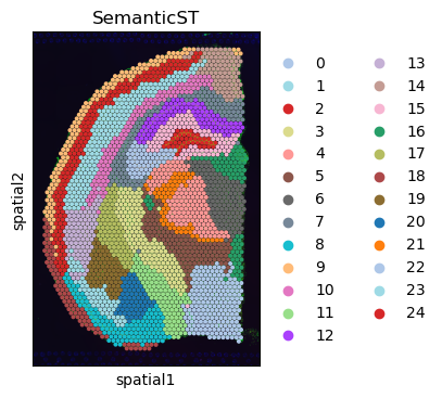
plt.rcParams["figure.figsize"] = (4, 4)
fig, ax = plt.subplots()
sc.pl.spatial(adata,  color="louvain",title='SemanticST',palette=adata.uns['colors'], ax=ax,size=1.5)
ax.axis('off')
plt.show()

WARNING: Length of palette colors is smaller than the number of categories (palette length: 22, categories length: 25. Some categories will have the same color.

Clustering

- Leiden

sc.tl.leiden(adata, resolution=0.9)
plt.rcParams["figure.figsize"] = (4, 4)
fig, ax = plt.subplots()
sc.pl.spatial(adata,  color="leiden",title='SemanticST',palette=adata.uns['colors'], ax=ax,size=1.5)
ax.axis('off')
plt.show()